Spectral analysis
Warning
These examples are out of date and may no longer work. Please refer first to the API Reference until the examples are updated.
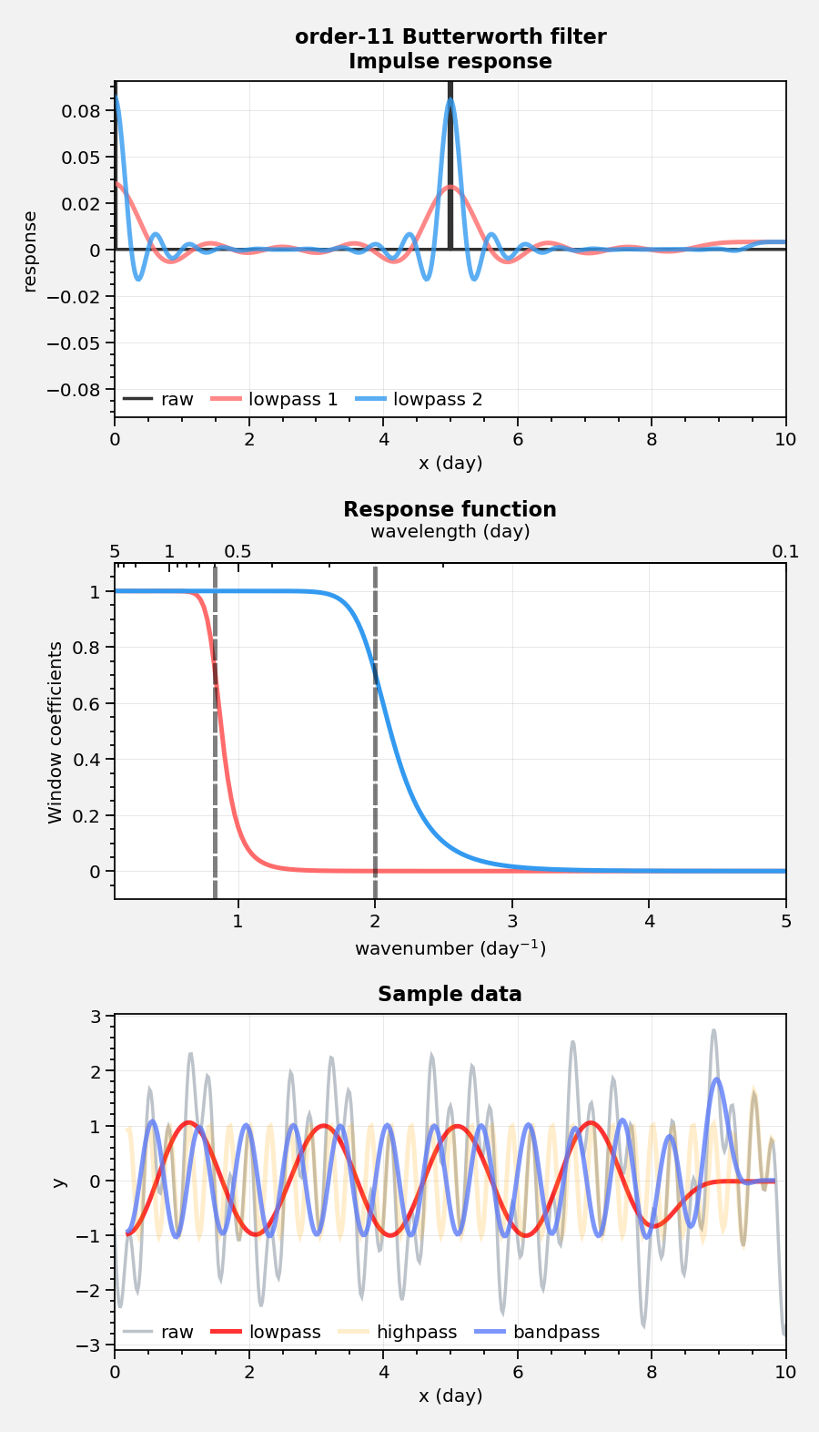
Spectral filtering
Use filter to filter data. Note this feature needs more
testing! But feel free to copy my code. The below shows response
functions and impulse response curves, and applies the filter to some
sample data.
import proplot as plot
import climopy as climo
import numpy as np
plot.nbsetup()
x = np.linspace(0,20,1000) # 20 days, but with tons of data in-between
d = climo.waves(x, wavelens=[1, 2])
# Fake data
n = 501
wsample = 10
cutoff = 1.2
cutoff2 = 0.5
waves = [0.3, 0.7, 2]
x = np.linspace(0,wsample,n) # 20 days, but with tons of data in-between
data = climo.waves(x, np.array(waves), phase=None)
# Iterate
filters = ['lanczos', 'butterworth']
# filters = ['butterworth', 'lanczos']
# filters = ['butterworth']
for filt in filters:
    # Create filters
    dx = x[1]-x[0]
    if filt=='lanczos':
        wfilter = 2
        w = climo.lanczos(dx, wfilter, cutoff)
        w2 = climo.lanczos(dx, wfilter, cutoff2)
        suptitle = f'{wfilter}-day Lanczos filter'
        # suptitle = f'{len(w[0])}-day Lanczos filter'
        # w, w2 = [w], [w2]
    elif filt=='butterworth':
        wfilter = 11 # should be odd-numbered
        w = climo.butterworth(dx, wfilter, cutoff)
        w2 = climo.butterworth(dx, wfilter, cutoff2)
        suptitle =  f'order-{len(w[1])} Butterworth filter'
    colors = ('red5', 'blue5')
    nf = 2 if filt=='butterworth' else 1 # in *this case*, for display purposes, need to prevent shifting to left or right
    # Preparation for drawing
    radians = False
    scale = 2*np.pi if radians else 1
    cutoffs = (cutoff,cutoff2)
    weights = (w,w2)
    # Draw stuff
    f, axs = plot.subplots(right=0.2, left=0.7, top=0.5, array=[[1],[0],[3],[4]], hratios=(1,-.25,1,1),
                           sharex=False, spany=False, hspace=.7, aspect=2)
    ax = axs[1]
    for ic,iw,color in zip(cutoffs,weights,colors):
        # s, r = climo.lanczos(width, ic, dx, response=True)
        s, r = climo.response(dx, *iw) # b and a coefficients, or maybe just b
        # print(s.max()), print(x.max())
        s = s*scale # optionally convert to radians
        r = r.copy()
        h = ax.plot(s, r, color=color, lw=2)
        ax.axvline(scale/ic, color='k', ls='--', lw=2, alpha=0.5) # the cutoff wavelenghs, converted to wavenumber
    xlim = [1e-1, 5]
    if not radians: # wavenumbers on x-axis
        xlocator = 1 # frequencies of interest
        xlabel = 'wavenumber (day$^{-1}$)'
        xformatter = None
    else: # frequency in radians on x-axis
        xlim[1] *= np.pi
        xlocator = plot.arange(0,np.pi*8,np.pi*0.5) # frequencies of interest
        xlabel = 'frequency (rad day$^{-1}$)'
        xformatter=plot.PiFormatter()
    ax.format(xscale='linear', xlim=xlim, xlocator=xlocator, xtickminor=False,
              xformatter=xformatter, ylim=(-.1,1.1),
              xlabel=xlabel, ylabel='Window coefficients') # frequency i.e. radians per time unit
    # xlocator = np.array([0.1, 0.5, 1, 5, 10])
    xlocator = np.array([0.1, 0.5, 1, 5])
    ax2 = ax.twinx()
    ax2.format(xscale='inverse', xlim=xlim,
               xlabel='wavelength (day)', xlocator=xlocator, title='Response function',
               xtickdir='in', # xticklabeldir='in',
               xtickminor=True, xgrid=True, xgridminor=False)
    ax2.xaxis.grid(False, which='major')
    ax2.title.update({'position':(0.5,1.1)})
    for tick in ax2.xaxis.majorTicks:
        tick.gridline.set_visible(False)
    # Impulse response
    ax = axs[0]
    idata = data.copy()
    idata[:] = 0
    idata[0] = 1
    idata[len(idata)//2] = 1
    ifilter = climo.filter(idata, *w, n=nf, axis=0, fix=False)
    ifilter2 = climo.filter(idata, *w2, n=nf, axis=0, fix=False)
    ax.plot(x, idata, color='k', label='raw', alpha=0.8)
    ax.plot(x, ifilter, color=colors[0], alpha=0.8, ls='-', lw=2, label='lowpass 1')
    ax.plot(x, ifilter2, color=colors[1], alpha=0.8, ls='-', lw=2, label='lowpass 2')
    ax.legend()
    ylim = max(np.nanmax(np.abs(ifilter)), np.abs(np.nanmax(ifilter2)))*1.1
    ax.format(xlim=(0,x.max()), suptitle=suptitle,
              xlabel='x (day)', ylabel='response', title='Impulse response', ylim=(-ylim, ylim))
    # Next play with sample data
    # Can show that, given some weights, lfilter does exact same thing as rolling() function
    # lanczos_roll = climo.rolling(data, w, axis=0)
    # lanczos_roll2 = climo.rolling(data, w2, axis=0)
    ax = axs[2]
    lfilter = climo.filter(data, *w, n=nf, axis=0) # with builtin signal method
    lfilter2 = climo.filter(data, *w2, n=nf, axis=0)
    ax.plot(x, data, color='gray5', label='raw', alpha=0.8)
    # ax.plot(x, lanczos_roll, color='r', alpha=1, ls='--', lw=2, label='Lanczos')
    # ax.plot(x, data-lanczos_roll2, color='orange', alpha=0.2, ls='-', lw=2, label='Lanczos')
    # ax.plot(x, lanczos_roll2-lanczos_roll, color='indigo5', alpha=1, ls='-', lw=2) # bandpass attempt
    ax.plot(x, lfilter, color='r', alpha=0.8, ls='-', lw=2, label='lowpass') # capture low-freq oscillation
    ax.plot(x, data - lfilter2, color='orange', alpha=0.2, ls='-', lw=2, label='highpass') # capture high-freq oscillation
    ax.plot(x, lfilter2 - lfilter, color='indigo5', alpha=0.8, ls='-', lw=2, label='bandpass') # capture middle oscillation
    ax.format(xlabel='x (day)', ylabel='y', title='Sample data',
              # ylim=(-.01,.01), yformatter=plot.Formatter(precision=3),
             )
    ax.legend(ncols=4)
    f.save(f'{filt}_display.pdf')

1D power spectra
Use the power function to get the spectral power. You can
use the exact same function for getting the co-spectra, quadrature
spectra, and individual power spectra for two different time series! The
below tests its performance with an artificial dataset consisting of 3
sine curves, generated with waves.
import proplot as plot
import climopy as climo
import numpy as np
plot.nbsetup()
x = np.linspace(0,100,10000) # 20 days
dx = x[1]-x[0]
# Data
# waves = [0.1, 0.2, 0.4, 0.6, 0.8, 3, 4, 5, 10, 30]
waves = [0.5, 1, 4]
window = len(x)//3 # 3 windows, or *5* overlapping windows
data = climo.waves(x, waves, phase=None)

# Spectrum
# freq, power = climo.power(data, dx, wintype=('gaussian',2000))
# freq, power = climo.power(data, dx, wintype='boxcar', nperseg=2000)
freq, power = climo.power(data, dx=dx, cyclic=False, manual=True, wintype='hann', nperseg=2000, scaling='spectrum')
freq = 1/freq # to wavelengths

# Figure
f, axs = plot.subplots(nrows=2, aspect=2, hspace=0.8, width=4, sharex=False, spany=False, hratios=(1,.5))
ax = axs[0]
ax.plot(x, data, label='raw')
ax.format(xlabel='x', ylabel='y', suptitle='Power spectra')
ax = axs[1]

# Plot
wnums = np.array([10, 0.3])
ax.plot(freq, power, label='power spectrum')
ax.format(xlim=1/wnums, xlabel='wavelength (days)', ylabel='strength')
var = data.var()
ax.text(-0.05, 1.5, f'total variance: {var:.1f}', va='top', weight='bold', transform='axes')
ax = ax.twiny()
ax.format(xlim=wnums[::-1], xscale='inverse', xlabel='wavenum (1/days)')
# ax.format(xlabel='wavelength (days)', ylabel='power (dB)', xscale='log', ylim=(-100,0))

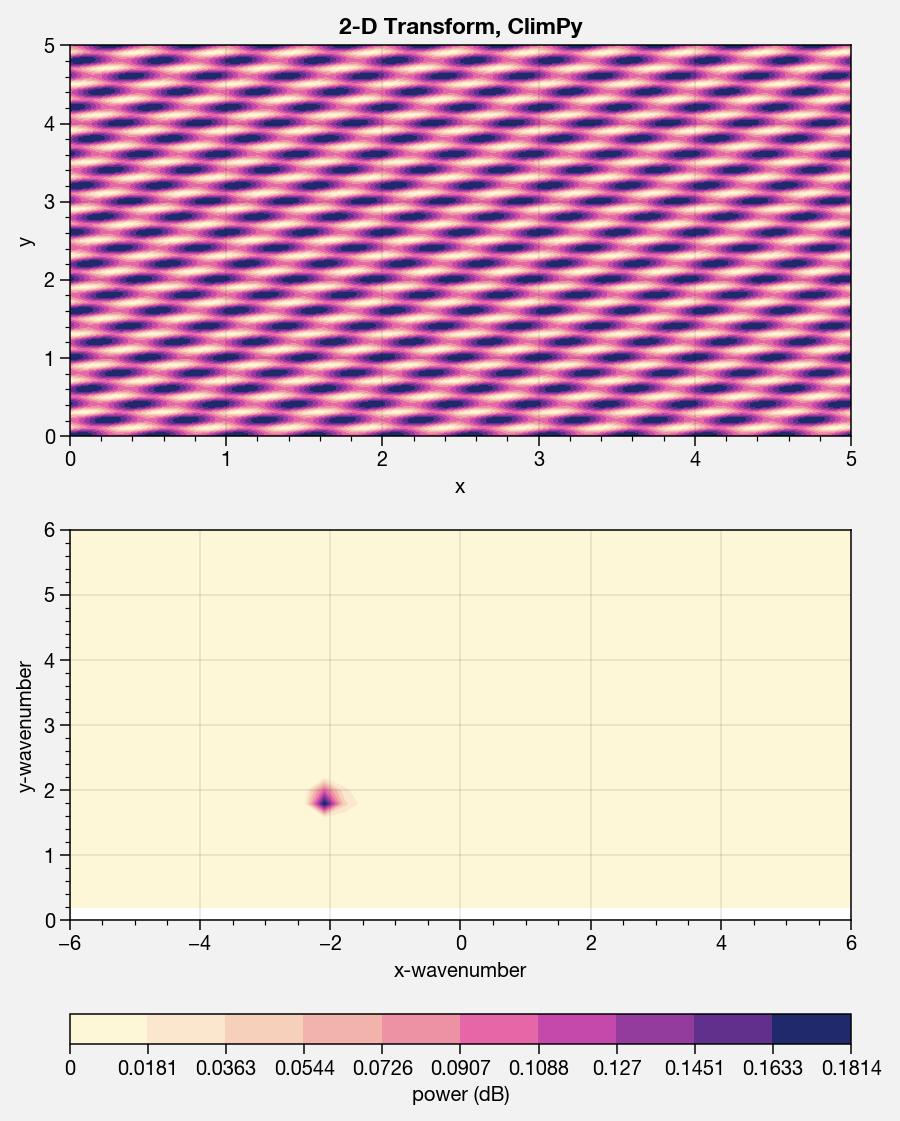
2D space-time power spectra
It’s also easy to get the “2-dimensional” spectral power, with one cyclic and one temporal axis, as in Randel and Held. The below demonstrates this ability with an artificial wavetrain propagating up the y axis with negative phase speed.
# Data
import proplot as plot
import climopy as climo
import numpy as np
plot.nbsetup()
n2 = 1800
n1 = int(n2*0.25)
n1 = int(n2*0.5)
nperseg = 600
x1 = np.linspace(0,5,n1) # cyclic dim
x2 = np.linspace(0,5,n2) # non-cyclic dims
offset = np.linspace(0,1.5*np.pi,n2)[::-1]
w1 = [2]
w2 = [5]
d1 = climo.waves(x1[:,None] + offset[None,:], w1)
d2 = climo.waves(x2[None,:], w2) # changing phase as we go up
dx1 = x1[1]-x1[0]
dx2 = x2[1]-x2[0]
data = d1 + d2
# Note: -2 transform will be transform of *real* data (i.e. symmetric), so left-half taken, but -1 transform
# will be transform of *complex* data, so both halves remain
f1, f2, result = climo.power2d(data, dx=dx1, dy=dx2, nperseg=nperseg, axes=(0,1))
fig, axs = plot.subplots(nrows=2, aspect=2, width=5, sharex=False, spany=False, bottomcolorbar=True)
# result = 10*np.log10(result)
ax = axs[0]
ax.contourf(x1, x2, data.T, cmap='sunset')
ax.format(suptitle='2-D Transform, ClimPy', xlabel='x', ylabel='y')
ax = axs[1]
m = ax.contourf(f1, f2, result.T, cmap='sunset', levels=np.linspace(result.min(),result.max(),11))
xl = 6
ylim = (0, 6)
ax.format(xlabel='x-wavenumber', ylabel='y-wavenumber', xlim=(-xl,xl), ylim=ylim)
fig.bottompanel.colorbar(m, clabel='power (dB)')